How to Draw Polinomial Linear Regression in R

In 1981, n = 78 bluegills were randomly sampled from Lake Mary in Minnesota. The researchers (Cook and Weisberg, 1999) measured and recorded the following data (Bluegills dataset):

• Response \(\left(y \right) \colon\) length (in mm) of the fish
• Potential predictor \(\left(x_1 \right) \colon \) age (in years) of the fish

The researchers were primarily interested in learning how the length of a bluegill fish is related to it age.

A scatter plot of the data:

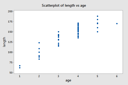
suggests that there is positive trend in the data. That is, not surprisingly, as the age of bluegill fish increases, the length of the fish tends to increase. The trend, however, doesn't appear to be quite linear. It appears as if the relationship is slightly curved.

One way of modeling the curvature in these data is to formulate a "second-order polynomial model" with one quantitative predictor:

\(y_i=(\beta_0+\beta_1x_{i}+\beta_{11}x_{i}^2)+\epsilon_i\)

where:

• \(y_i\) is length of bluegill (fish) \(i\) (in mm)
• \(x_i\) is age of bluegill (fish) \(i\) (in years)

and the independent error terms \(\epsilon_i\) follow a normal distribution with mean 0 and equal variance \(\sigma^{2}\).

You may recall from your previous studies that "quadratic function" is another name for our formulated regression function. Nonetheless, you'll often hear statisticians referring to this quadratic model as a second-order model, because the highest power on the \(x_i\) term is 2.

Incidentally, observe the notation used. Because there is only one predictor variable to keep track of, the 1 in the subscript of \(x_{i1}\) has been dropped. That is, we use our original notation of just \(x_i\). Also note the double subscript used on the slope term, \(\beta_{11}\), of the quadratic term, as a way of denoting that it is associated with the squared term of the one and only predictor.

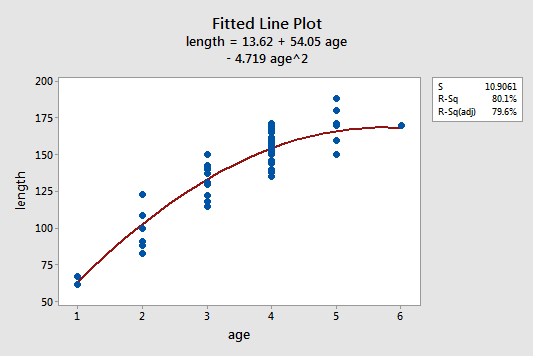
The estimated quadratic regression function looks like it does a pretty good job of fitting the data:

To answer the following potential research questions, do the procedures identified in parentheses seem reasonable?

• How is the length of a bluegill fish related to its age? (Describe the nature — "quadratic" — of the regression function.)
• What is the length of a randomly selected five-year-old bluegill fish? (Calculate and interpret a prediction interval for the response.)

Among other things, the Minitab output:

Analysis of Variance

Source	DF	Adj SS	Adj MS	F-Value	P-Value
Regression	2	35938.0	17969.0	151.07	0.000
age	1	8252.5	8252.5	69.38	0.000
age^2	1	2972.1	2972.1	24.99	0.000
Error	75	8920.7	118.9
Lack-of-Fit	3	108.0	360	0.29	0.829
Pure Error	72	88121.7	122.4
Total	77	44858.7

Model Summary

S	R-sq	R-sq(adj)	R-sq(pred)
10.9061	80.11%	79.58%	78.72%

Coefficients

Term	Coef	SE Coef	T-Value	P-Value	VIF
Constant	13.6	11.0	1.24	0.220
age	54.05	6.49	8.33	0.000	23.44
age^2	-4.719	0.944	-5.00	0.000	23.44

Regression Equation

length = 13.6 + 54.05 age - 4.719 age^2

Predictions for length

Variable	Setting
age	5
age^2	25

Fit	SE Fit	95% CI	95% PI
165.902	2.76901	(160.386, 171.418)	(143.487, 188.318)

tells us that:

• 80.1% of the variation in the length of bluegill fish is reduced by taking into account a quadratic function of the age of the fish.
• We can be 95% confident that the length of a randomly selected five-year-old bluegill fish is between 143.5 and 188.3 mm.

How to Draw Polinomial Linear Regression in R

Source: https://online.stat.psu.edu/stat501/lesson/9/9.8

Share this post